Optimization
Overview
Global optimization searches the entire solution space of a given problem to get the best possible match to a set of desired conditions. Our solver takes your target kinematic curves and a set of boundary conditions on the points and searches for the best possible configuration.
As with most mathematical optimizations the boundary conditions have a very strong influence on the outcome and should be set carefully and specifically to your desired outcome. Some good strategies are:
Allow enough freedom in the boundary conditions. For example, allowing only a single point to move or restricting point limits to only a very small distance will result in the total solution space being quite small and likely similar to the starting conditions. This may prevent any close solution from being found.
Restrict boundary conditions where needed. Restrict your boundary conditions to realistic limits to prevent the solver honing in on unrealistic point positions (such as pivots behind the axle). Sometimes it can be helpful to run several low resolution studies and progressively restrict point movement in line with your intended design direction.
Run more low resolution solves. Solve times are much quicker for lower resolution solves but not necessarily less accurate. It is almost always advantageous to run several fast solves to understand where the results are being driven and alter boundary conditions as needed before further optimization.
Run a Study
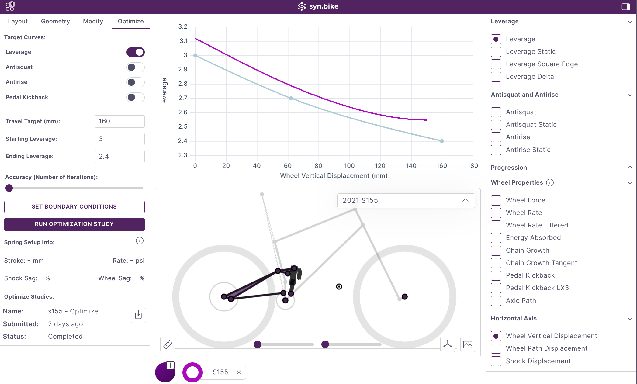
Set Target Curves
Target curves can be set for the 4 primary kinematic metrics: Vertical Leverage, Antisquat, Antirise, and Pedal Kickback. Select the target or set of targets you want to use from the list under the Optimize tab. A default target curve will be generated for each selection.
The target travel and starting leverage must be set manually and then the handles of the curve can be dragged to set the target shape. Additional curve handles can be created and removed by double clicking on the curve.
Configure Boundary Conditions
Boundary conditions define how much each kinematic point is allowed to move during optimization. For each point you can set:
Fixed: The point will not move at all. Use this for points that must remain in their current position, such as main pivot locations on an existing frame.
Free: The point can move anywhere within the specified range. Set minimum and maximum values for both X and Y coordinates to define the allowable region.
To configure boundary conditions, expand the Boundary Conditions section in the Optimize tab. Each kinematic point will be listed with controls to set its movement constraints.
Tip: Start with generous boundary conditions and progressively tighten them based on results. This helps you understand which points have the most influence on your target curves.
Run Study and Review Results
Once your target curves and boundary conditions are configured:
Set the resolution: Higher resolution provides more accurate results but takes longer to compute. Start with a lower resolution for initial exploration.
Click Run: The solver will begin searching for the optimal point configuration. When complete you will see the status update and it will be available to load into the UI.
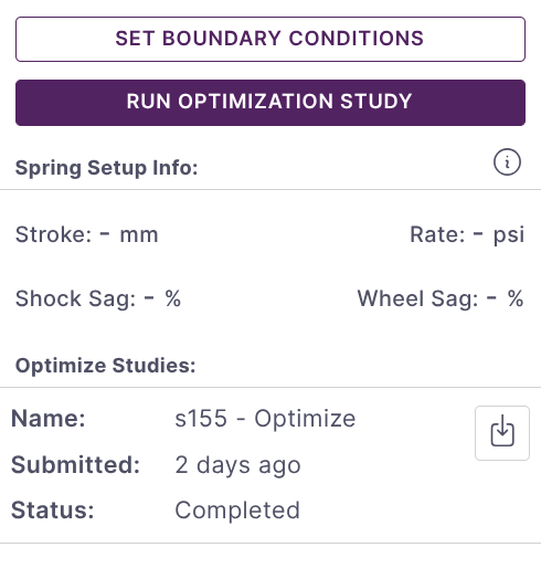
- Review results: Once loaded the optimized configuration will be shown as a new model. If you are happy with the results the name can be updated and the model saved to override the previous version or as a new version.
If the results don't meet your expectations, consider:
- Adjusting boundary conditions to allow more or less freedom
- Modifying target curves to be more achievable
- Running additional studies with different starting configurations
Tips for Effective Optimization
Choosing Target Curves
Not all curve combinations are physically achievable. Some guidelines:
- Leverage alone is usually the easiest to optimize and a good starting point.
- Leverage + Antisquat is a common combination that works well for some linkage types. Note that antisquat curve shape is inherently coupled to the chosen suspension layout. While changing the offset of the antisquat curve is possible, often changing the curve shape is not.
- Adding Antirise increases complexity and may require more freedom in boundary conditions.
- Pedal Kickback is highly dependent on axle path and may conflict with other targets. Generally not recommended.
Understanding Trade-offs
The optimizer finds the best compromise between all selected targets. If you're not getting good results on one metric, it may be because achieving that target conflicts with another. Try running separate studies with individual targets to understand what's achievable for each metric independently.
Iterative Refinement
Studies are non-deterministic meaning different runs with the same input conditions may yield better or worse results. When exploring it may be worth running several studies to see what the initial sensitivity is like.
The most effective approach is iterative:
- Run a quick, low-resolution study with broad boundary conditions
- Analyze which points moved significantly and in what direction
- Tighten boundary conditions around promising regions
- Run a higher resolution study
- Repeat until satisfied with the results